Multifield Transformations: Many-to-One and One-to-Many Field Mapping
Verified Concept Article • Factual Traceability Enabled
Summary OverviewMultifield transformations map multiple source fields to a single target field or a single source field to multiple target fields within ETL processes.
Home > ## ETL modelling - Overview > Field Mapping Strategies in Data Transformation > Multifield Transformations: Many-to-One and One-to-Many Field Mapping
Detailed Explanation
In data‑warehouse environments, the transformation phase of the ETL (Extract, Transform, Load) pipeline is where raw operational data is reshaped to fit the analytical schema of the target system. While single‑field transformations apply a function to a solitary column, multifield transformations involve a relational mapping between sets of fields. The literature distinguishes two canonical patterns: a many‑to‑one (M:1) mapping, where several source attributes are combined into a single destination attribute, and a one‑to‑many (1:M) mapping, where one source attribute is decomposed into several derived columns.
The many‑to‑one case often arises during joining or aggregation operations. For example, a customer’s first name, middle name, and last name—stored in separate source fields—may be concatenated into a single "FullName" column in the data warehouse. Similarly, numeric fields such as "UnitsSold" and "UnitPrice" can be summed or multiplied to produce a composite metric like "Revenue". This process aligns with the "joining – data combining" step described in source [3], where multiple fields are merged to create a richer representation.
Conversely, the one‑to‑many pattern is typical of splitting or derived‑field generation. A single timestamp field might be partitioned into separate "Date", "Hour", and "Minute" columns to support time‑based slicing. Another common scenario is extracting hierarchical components from a coded identifier—e.g., separating a product code "ABC‑123" into a category code "ABC" and an item number "123". The source material on page 26 explicitly labels this as "1:M – from one source field to many target fields" (source [1]), underscoring its role in expanding the granularity of analytical dimensions.
Both patterns are integral to the broader field mapping strategies that ensure semantic consistency across heterogeneous source systems. They are implemented via algorithmic formulas, logical expressions, or table lookups, as outlined for single‑field transformations in source [2]; the same mechanisms extend naturally to multifield contexts, albeit with additional logic to coordinate multiple inputs or outputs.
Examples
Consider a retail data feed that includes separate fields for "Street", "City", "State", and "ZIP". A many‑to‑one transformation would concatenate these into a unified "Address" column, often using a delimiter such as a comma and space. The transformation function might be expressed in SQL as CONCAT(Street, ', ', City, ', ', State, ' ', ZIP). This aggregated address simplifies downstream reporting where a single address string is sufficient.
In a one‑to‑many example, a source field "FullDateTime" stored as an ISO‑8601 string (e.g., "2023-07-15T14:30:00Z") can be split into three target fields: "Date" (2023-07-15), "Time" (14:30:00), and "Timezone" (Z). The extraction can be performed using substring functions or date‑time parsing libraries. This decomposition enables analysts to filter by date without parsing the full timestamp each time.
A further illustration of many‑to‑one aggregation appears in financial consolidation: the fields "RevenueQ1", "RevenueQ2", "RevenueQ3", and "RevenueQ4" are summed to produce an annual "TotalRevenue" column. Conversely, a one‑to‑many decomposition might involve a composite key "RegionProduct" (e.g., "EMEAWidget") that is split into distinct "Region" and "Product" columns, facilitating region‑level and product‑level analytics.
These examples demonstrate how multifield transformations serve as the connective tissue between operational data structures and the dimensional models required for robust business intelligence.
Visual References from Cited Pages
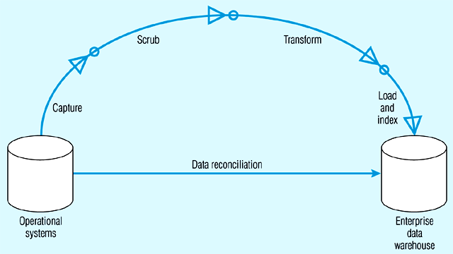
Figure 1: Illustration of data reconciliation stepsSource: ETLmodelling.pdf (Page 21)
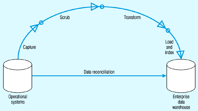
Figure 2: Data reconciliation steps diagramSource: ETLmodelling.pdf (Page 24)
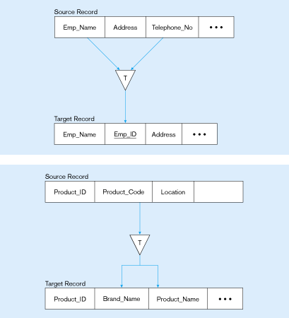
Figure 3: Multifield transformationSource: ETLmodelling.pdf (Page 26)
Incoming Backlinks
Other pages in this wiki that link back to the current topic.